Korean J Radiol.  2020 Jan;21(1):33-41. 10.3348/kjr.2019.0312.

Basics of Deep Learning: A Radiologist's Guide to Understanding Published Radiology Articles on Deep Learning

• Do S
• Song KD
• Chung JW

• KMID: 2467040
• DOI: http://doi.org/10.3348/kjr.2019.0312

Abstract

Artificial intelligence has been applied to many industries, including medicine. Among the various techniques in artificial intelligence, deep learning has attained the highest popularity in medical imaging in recent years. Many articles on deep learning have been published in radiologic journals. However, radiologists may have difficulty in understanding and interpreting these studies because the study methods of deep learning differ from those of traditional radiology. This review article aims to explain the concepts and terms that are frequently used in deep learning radiology articles, facilitating general radiologists' understanding.

Keyword

Artificial intelligence; Deep learning; Convolutional neural network; Radiology

MeSH Terms

Artificial Intelligence
Diagnostic Imaging
Learning*

Figure

• 

  Fig. 1 Diagram of artificial intelligence hierarchy. Machine learning is field of study that gives computers ability to learn without being explicitly programmed. Deep learning is subset of machine learning that makes computation of multi-layer neural networks feasible. CNN is subset of deep learning characterized by convolutional layer. CNN = convolutional neural network

• 

  Fig. 2 Schematic diagram of CNN model and other regular neural networks. A. CNN includes convolutional layers, pooling layers, and fully connected layers. B. Each layer is fully connected to all neurons in next layer in other regular neural networks. Conv = convolution

• 

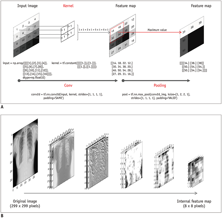
  Fig. 3 Convolution and pooling. A. Example of convolution and pooling. Convolution implies that kernel is applied to input image to produce feature map. Pooling is down-sampling operation. Input, kernel, and feature map are all expressed by matrices, and convolution and pooling are both matrix operations. In this example, a kernel (2 × 2) is applied across input data and element-wise product between kernel and input data is first calculated at each location and then summed to obtain output value in corresponding position of feature map (1 × 1 + 2 × 1 + 5 × 1 + 6 × 1 = 14). In pooling operation, max pooling with filter size of 2 × 2 is applied. Among four values (14, 18, 30, and 34), maximum value (34) is output in corresponding position of next layer. B. Visualization of feature maps through multi-step convolution and pooling. Example of visualized feature maps with chest radiographic image as input for task to differentiate between abdominal and chest radiographs.

• 

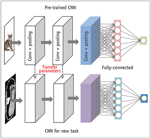
  Fig. 4 Transfer learning. Transfer learning is process of taking pre-trained model (usually trained on large dataset, such as ImageNet) and “fine-tuning” model with new dataset. Fully connected layers, with or without parts of kernels of convolutional layers of pre-trained model are replaced with new set and are trained with dataset of new task.

• 

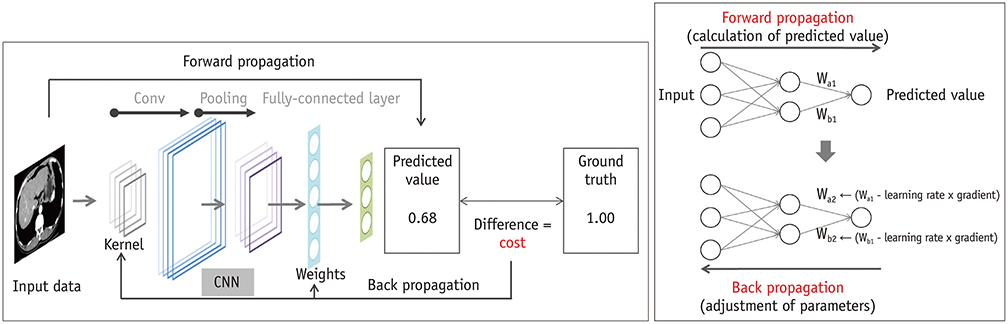
  Fig. 5 Model training. Model training is process of parameter (kernel + weight) optimization through forward and back propagation. Forward propagation is process used to calculate predicted value from input data through model. Back propagation is process used to adjust each parameter of model toward minimizing cost. When presenting series of training samples to model, difference between predicted value and ground truth (target class or regression value) is measured using cost function. Using gradient descent method, all parameters (weights in fully connected layer and kernels in convolutional layer) are slightly adjusted to minimize cost.

• 

  Fig. 6 Gradient descent. Gradient descent is optimization algorithm used to identify parameters that minimize cost. Parameter is repeatedly updated until cost reaches minimum with following formula: Wb = Wa − (learning rate) × (gradient). Optimal parameter of model is value that minimizes cost most. In graph (A), gradient is negative at initial value of parameter (a), and value of (− learning rate × gradient at Wa) is positive. As result, parameter is updated toward increasing value. By repeating this process, minimum of cost function (c) can be obtained, which is parameter's optimal value. On the other hand, gradient is positive at initial value of parameter (a) in graph (B) and value of (− learning rate × gradient at Wa) is negative. As result, parameter is updated in direction of decreasing value, and minimum of cost function (c) is reached. Using gradient descent method, parameter can be optimized regardless of parameter's initial value (initial values of parameters are commonly randomly set). Letter “W” is derived from weight and weight is same as parameter in this case.

• 

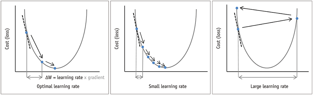
  Fig. 7 Effect of learning rate on model training. Learning rate is hyperparameter that determines degree of parameter update. It is important to set learning rate to appropriate value. If learning rate is too small, model will converge too slowly. On the other hand, if learning rate is too large, model will diverge without convergence. Letter “W” is derived from weight and weight is same as parameter in this case.

• 

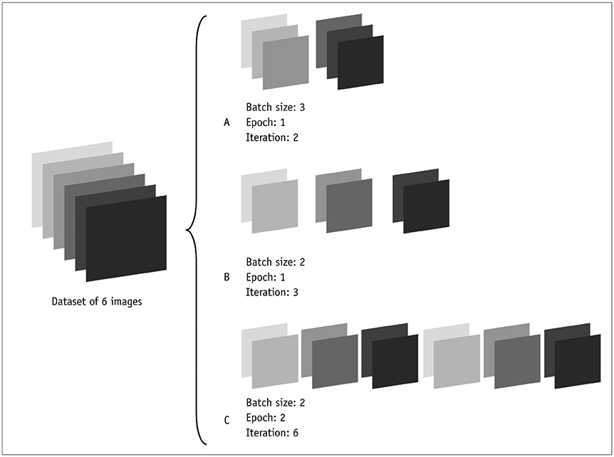
  Fig. 8 Epoch, batch, and iteration. There is dataset of 6 images. In C, batch size is 2, and algorithm is set to run for 2 epochs. Therefore, in each epoch, there are 3 batches (6 / 2 = 3). Each batch gets passed through algorithm, so there are 3 iterations per epoch. Since 2 epochs were specified, there are total of 6 iterations (3 × 2 = 6) for training. In A, batch size, epoch, and iteration are 3, 1, and 2, respectively. In B, batch size, epoch, and iteration are 2, 1, and 3, respectively.

• 

  Fig. 9 Dice score and Jaccard index. FN = false negative, FP = false positive, TN = true negative, TP = true positive

Reference

1. Chartrand G, Cheng PM, Vorontsov E, Drozdzal M, Turcotte S, Pal CJ, et al. Deep learning: a primer for radiologists. Radiographics. 2017; 37:2113–2131.

2. Litjens G, Kooi T, Bejnordi BE, Setio AAA, Ciompi F, Ghafoorian M, et al. A survey on deep learning in medical image analysis. Med Image Anal. 2017; 42:60–88.

3. Dreyer KJ, Geis JR. When machines think: radiology’s next frontier. Radiology. 2017; 285:713–718.

4. Soffer S, Ben-Cohen A, Shimon O, Amitai MM, Greenspan H, Klang E. Convolutional neural networks for radiologic images: a radiologist's guide. Radiology. 2019; 290:590–606.

5. Cardoso JR, Pereira LM, Iversen MD, Ramos AL. What is gold standard and what is ground truth? Dental Press J Orthod. 2014; 19:27–30.

6. Zhong Z, Zheng L, Kang G, Li S, Yang Y. Random erasing data augmentation. eprint arXiv;2017. Accessed April 1, 2019. Available at: https://ui.adsabs.harvard.edu/abs/2017arXiv170804896Z.

7. TIOBE index for April 2019. TIOBE Web site;Accessed April 30, 2019. https://www.tiobe.com/tiobe-index/.

8. Jia Y, Shelhamer E, Donahue J, Karayev S, Long J, Girshick R, et al. Caffe: convolutional architecture for fast feature embedding. eprint arXiv;2014. Accessed April 1, 2019. Available at: https://ui.adsabs.harvard.edu/abs/2014arXiv1408.5093J.

9. Bastien F, Lamblin P, Pascanu R, Bergstra J, Goodfellow I, Bergeron A, et al. Theano: new features and speed improvements. eprint arXiv;2012. Accessed April 1, 2019. Available at: https://ui.adsabs.harvard.edu/abs/2012arXiv1211.5590B.

10. Abadi M, Barham P, Chen J, Chen Z, Davis A, Dean J, et al. TensorFlow: a system for large-scale machine learning. eprint arXiv;2016. Accessed April 1, 2019. Available at: https://ui.adsabs.harvard.edu/abs/2016arXiv160508695A.

11. Lee JG, Jun S, Cho YW, Lee H, Kim GB, Seo JB, et al. Deep learning in medical imaging: general overview. Korean J Radiol. 2017; 18:570–584.

12. Krizhevsky A, Sutskever I, Hinton GE. ImageNet classification with deep convolutional neural networks. Advances in Neural Information Processing Systems. 2012; 25:1090–1098.

13. Lee C, Kim Y, Kim YS, Jang J. Automatic disease annotation from radiology reports using artificial intelligence implemented by a recurrent neural network. AJR Am J Roentgenol. 2019; 212:734–740.

14. Girshick R, Donahue J, Darrell T, Malik J. Rich feature hierarchies for accurate object detection and semantic segmentation. eprint arXiv;2013. Accessed April 1, 2019. Available at: https://ui.adsabs.harvard.edu/abs/2013arXiv1311.2524G.

15. Kazuhiro K, Werner RA, Toriumi F, Javadi MS, Pomper MG, Solnes LB, et al. Generative adversarial networks for the creation of realistic artificial brain magnetic resonance images. Tomography. 2018; 4:159–163.

16. Goodfellow IJ, Pouget-Abadie J, Mirza M, Xu B, Warde-Farley D, Ozair S, et al. Generative adversarial networks. eprint arXiv;2014. Accessed April 1, 2019. Available at: https://ui.adsabs.harvard.edu/abs/2014arXiv1406.2661G.

17. Ronneberger O, Fischer P, Brox T. U-net: convolutional networks for biomedical image segmentation. eprint arXiv;2015. Accessed April 1, 2019. Available at: https://ui.adsabs.harvard.edu/abs/2015arXiv150504597R.

18. Huang G, Liu Z, van der Maaten L, Weinberger KQ. Densely connected convolutional networks. eprint arXiv;2016. Accessed April 1, 2019. Available at: https://ui.adsabs.harvard.edu/abs/2016arXiv160806993H.

19. Simonyan K, Zisserman A. Very deep convolutional networks for large-scale image recognition. eprint arXiv;2014. Accessed April 1, 2019. Available at: https://ui.adsabs.harvard.edu/abs/2014arXiv1409.1556S.

20. He K, Zhang X, Ren S, Sun J. Deep residual learning for image recognition. eprint arXiv;2015. Accessed April 1, 2019. Available at: https://ui.adsabs.harvard.edu/abs/2015arXiv151203385H.

21. Szegedy C, Liu W, Jia Y, Sermanet P, Reed S, Anguelov D, et al. Going deeper with convolutions. eprint arXiv;2014. Accessed April 1, 2019. Available at: https://ui.adsabs.harvard.edu/abs/2014arXiv1409.4842S.

22. He K, Gkioxari G, Dollár P, Girshick R. Mask R-CNN. eprint arXiv;2017. Accessed April 1, 2019. Available at: https://ui.adsabs.harvard.edu/abs/2017arXiv170306870H.

23. Lecun Y, Bottou L, Bengio Y, Haffner P. Gradient-based learning applied to document recognition. Proceedings of the IEEE. 1998; 86:2278–2324.

24. Zeiler MD, Fergus R. Visualizing and understanding convolutional networks. eprint arXiv;2013. Accessed April 1, 2019. Available at: https://ui.adsabs.harvard.edu/abs/2013arXiv1311.2901Z.

25. Qian N. On the momentum term in gradient descent learning algorithms. Neural Netw. 1999; 12:145–151.

26. Nesterov YE. A method for solving the convex programming problem with convergence rate O(1/k²). Dokl Akad Nauk SSSR. 1983; 269:543–547.

27. Duchi J, Hazan E, Singer Y. Adaptive subgradient methods for online learning and stochastic optimization. J Mach Learn Res. 2011; 12:2121–2159.

28. Zeiler MD. ADADELTA: an adaptive learning rate method. eprint arXiv;2012. Accessed April 1, 2019. Available at: https://ui.adsabs.harvard.edu/abs/2012arXiv1212.5701Z.

29. Kingma DP, Ba J. Adam: a method for stochastic optimization. eprint arXiv;2014. Accessed April 1, 2019. Available at: https://ui.adsabs.harvard.edu/abs/2014arXiv1412.6980K.